Flow fields#
A* is a single-source single-destination graph search that uses heuristics to find the path quicker. If many agents are finding paths to the same destination, or if many agents are finding paths from the same starting point, it is often faster to use Dijsktra’s Algorithm once than to use A* many times. If the movement costs don’t vary, Breadth First Search[1] runs even faster.
Dijsktra’s Algorithm and Breadth First Search produce not only a path but also a field which is a value at every point. There are two types of fields these algorithms can produce:
- A distance field is a number at every location that tells you the distance to a location. In the roguelike game community these are called Dijkstra maps[2]. They can be used to calculate Influence maps[3].
- A flow field is a direction at every location that tells you the direction to go to move towards a location.
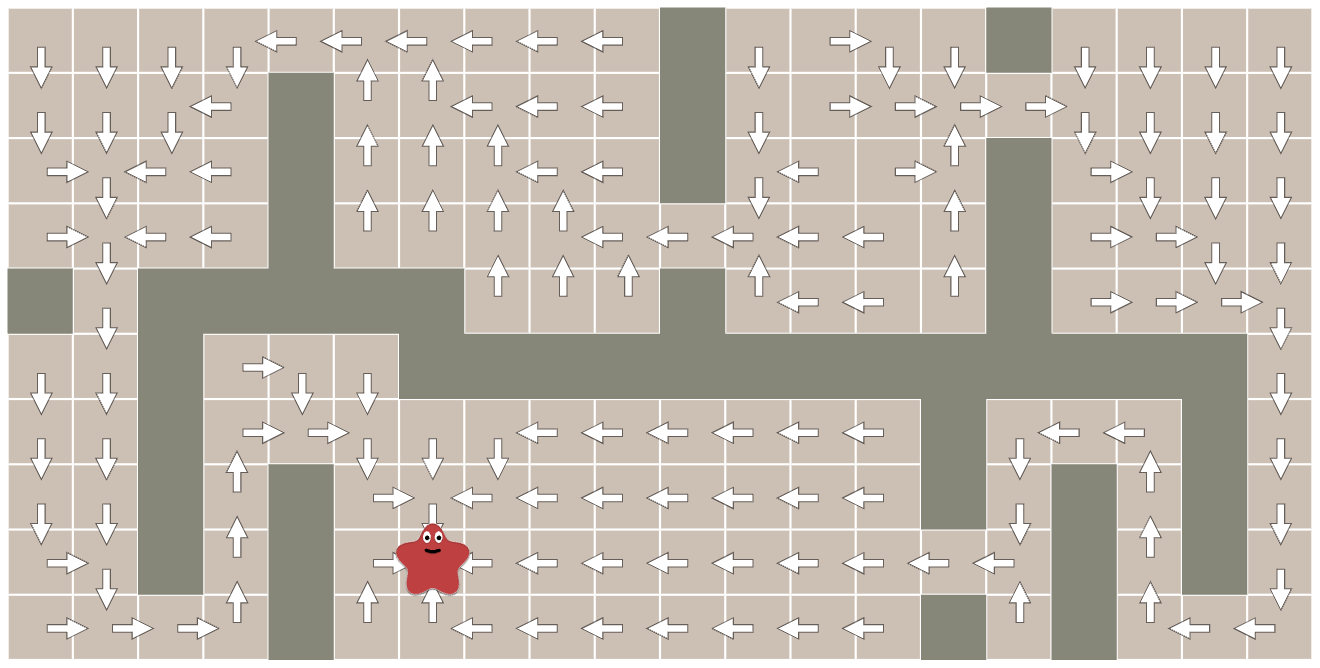 Flow Field
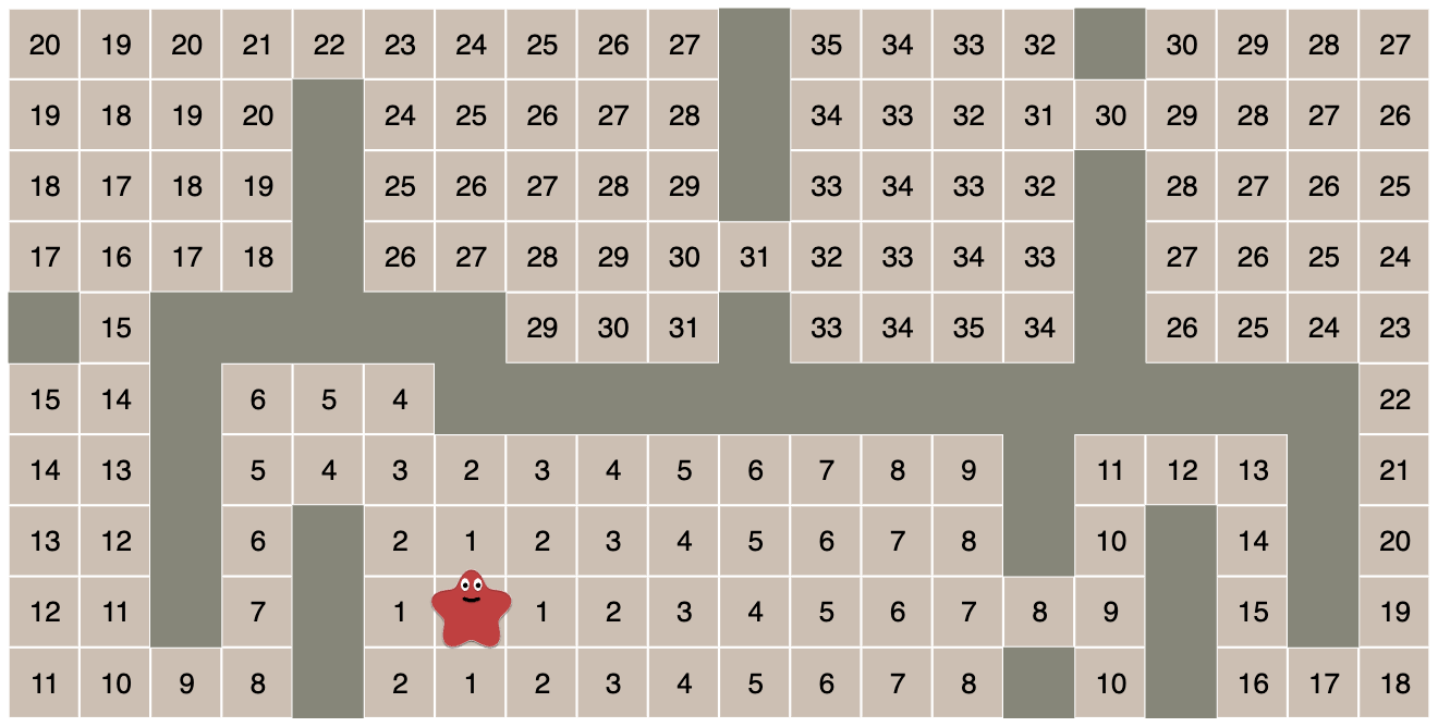 Distance Field
In the code I
present on my interactive A* page[4], the cost_so_far variable is
the distance field and the came_from variable is the flow
field. These two are related. In vector calculus, the flow field is
the negative gradient (∇) of the distance field. You can store the
distance field and then calculate the flow field by looking at which
neighbor has the lowest distance.
When agent movement is continuous instead of discrete, use interpolation between adjacent nodes to calculate the flow at a specific point.
Distance and flow fields can be combined with approaches to store multiple levels of granularity.
Flow fields can be combined with fields representing crowding to have agents spread out instead of colliding with each other. Look for research papers on continuum crowds[5] (PDF), or see this overview[6].
Flow fields calculated with Dijkstra’s Algorithm use the graph distance. If movement is any-angle then Euclidean distance will produce a more accurate flow field. The Fast Marching Method[7] is a modification of Dijkstra’s Algorithm to calculate the Euclidean distance instead of the graph distance. A different approach is taken by Replacement Product Graphs[8], which modifies the graph to make graph distance closer to Euclidean distance.
Beam search#
In the main A* loop, the OPEN set stores all the nodes that may need to be searched to find a path. The Beam Search is a variation of A* that places a limit on the size of the OPEN set. If the set becomes too large, the node with the worst chances of giving a good path is dropped. One drawback is that you have to keep your set sorted to do this, which limits the kinds of data structures you’d choose.
Iterative deepening#
Iterative Deepening is an approach used in many AI algorithms to start
with an approximate answer, then make it more accurate. The name
comes from game tree searches, where you look some number of moves
ahead (for example, in Chess). You can try to deepen the tree by
looking ahead more moves. Once your answer doesn’t change or improve
much, you assume that you have a pretty good answer, and it won’t
improve when you try to make it more accurate again. In IDA*, the
“depth” is a cutoff for f values. When the f value is
too large, the node won’t even be considered (i.e., it won’t be
added to the OPEN set). The first time through you process very few
nodes. Each subsequent pass, you increase the number of nodes you
visit. If you find that the path improves, then you continue to
increase the cutoff; otherwise, you can stop. For more details, read
these
lecture nodes on IDA*[9].
I personally don’t see much need for IDA* for finding paths on game maps. ID algorithms tend to increase computation time while reducing memory requirements. In map pathfinding, however, the “nodes” are very small—they are simply coordinates. I don’t see a big win from not storing those nodes.
Weighted A*#
In games we often multiply the heuristic by some constant factor to
make A* run faster. This is called Weighted A* in the
literature. We can use some weight w > 1 (for example, 1.5 or
2.0) to increase the heuristic’s effect:
f(p) = g(p) + w * h(p)
This seems to work well in practice in most cases. Wilt and Ruml’s AAAI 2012 paper When does Weighted A* fail?[10] shows some situations where it doesn’t.
Another way to think about this is that Dijsktra’s Algorithm uses only
g and Greedy Best First Search uses only h. The weight
is a way to smoothly interpolate between these two algorithms, where a
weight of 0 means Dijkstra’s Algorithm and a weight of ∞ means Greedy
Best First Search. A weight of 1.0 is halfway between the two
extremes, giving A*. Weighted A* is in between A* and Greedy Best
First Search.
If the heuristic is too low only on some parts of the path or some parts of the map, we can use dynamic weighting:
f(p) = g(p) + w(p) * h(p)
There could be many ways to change the weight, but I didn’t explore this topic when I wrote these pages in 1997. At the time my intuition led me to believe that it’d be better to use a higher weight near the beginning of the path and a lower weight near the end. That is because I believed the weight compensated for the heuristic being too low, and it is typically too low at the beginning of the path and reasonably accurate near the end of the path. However, research has shown that my intuition was wrong. It’s better to apply the weight near the end of the path.
Chen and Sturvetant’s AAAI 2021 paper Necessary and Sufficient Conditions for Avoiding Reopenings in Best First Suboptimal Search with General Bounding Functions[11] presents two approaches, pxWU, which decreases the weight as you near the goal:
f(p) = g(p) < (2*w - 1) * h(p)
     ? g(p) / (2*w - 1) + h(p)
     : (g(p) + h(p)) / w
and pxWD, which increases the weight as you near the goal:
f(p) = g(p) < h(p)
     ? g(p) + h(p)
     : (g(p) + (2*w - 1) * h(p)) / w}
They found that increasing the weight works better. They also have an interactive demo[12] where you can try different weighting schemes.
Bandwidth search#
There are two properties about Bandwidth Search that some
people may find useful. This variation assumes that h is
an overestimate, but that it doesn’t overestimate by more than
some number e. If this is the case in your search, then
the path you get will have a cost that doesn’t exceed the best path’s
cost by more than e. Once again, the better you make
your heuristic, the better your solution will be.
Another property you get is that if you can drop some nodes in the
OPEN set. Whenever h+d is greater then the true cost of
the path (for some d), you can drop any node that has an
f value that’s at least e+d higher than the
f value of the best node in OPEN. This is a strange
property. You have a “band” of good values for f;
everything outside this band can be dropped, because there is a
guarantee that it will not be on the best path.
Curiously, you can use different heuristics for the two properties, and things still work out. You can use one heuristic to guarantee that your path isn’t too bad, and another one to determine what to drop in the OPEN set.
Note: When I wrote this in 1997, Bandwidth search looked potentially useful, but I’ve never used it and I don’t see much written about it in the game industry, so I will probably remove this section. You can search Google for more information[13], especially from textbooks.
Bidirectional search#
Instead of searching from the start to the finish, you can start two searches in parallel—one from start to finish, and one from finish to start. When they meet, you should have a good path.
It’s a good idea that will help in some situations. The idea behind bidirectional searches is that searching results in a “tree” that fans out over the map. A big tree is much worse than two small trees, so it’s better to have two small search trees.
The front-to-front variation links the two searches together.
Instead of choosing the best forward-search node—g(start,x) +
h(x,goal)—or the best backward-search node—g(y,goal) +
h(start,y)—this algorithm chooses a pair of nodes with the best g(start,x) + h(x,y) + g(y,goal).
The retargeting approach abandons simultaneous searches in the forward and backward directions. Instead, it performs a forward search for a short time, chooses the best forward candidate, and then performs a backward search—not to the starting point, but to that candidate. After a while, it chooses a best backward candidate and performs a forward search from the best forward candidate to the best backward candidate. This process continues until the two candidates are the same point.
Bidirectional search is easy to implement incorrectly. Everyone Gets Bidirectional BFS Wrong[14] about Breadth First Search}
Holte, Felner, Sharon, Sturtevant’s 2016 paper Front-to-End Bidirectional Heuristic Search with Near-Optimal Node Expansions[15] is a recent result with a near-optimal bidirectional variant of A*. Pijls and Post’s 2009 paper Yet another bidirectional algorithm for shortest paths[16] proposes an unbalanced bidirectional A* that runs faster than balanced bidirectional search. Sadhukhan’s 2013 paper Bidirectional heuristic search based on error estimate proposes tracking the difference between heuristic values and true costs to balance the forward and backward parts of bidirectional A* search.[17]
Dynamic A* and Lifelong Planning A*#
There are variants of A* that allow for changes to the world after the initial path is computed. D* is intended for use when you don’t have complete information. If you don’t have all the information, A* can make mistakes; D*’s contribution is that it can correct those mistakes without taking much time. LPA* is intended for use when the costs are changing. With A*, the path may be invalidated by changes to the map; LPA* can re-use previous A* computations to produce a new path.
However, both D* and LPA* require a lot of space—essentially
you run A* and keep around its internal information (OPEN/CLOSED sets, path tree, g values), and then when the map
changes, D* or LPA* will tell you if you need to adjust your path to
take into account the map changes.
For a game with lots of moving units, you usually don’t want to keep all that information around, so D* and LPA* aren’t applicable. They were designed for robotics, where there is only one robot—you don’t need to reuse the memory for some other robot’s path. If your game has only one or a small number of units, you may want to investigate D* or LPA*.
Additional variants I haven’t looked at yet: Focused D*, D* Lite
Jump Point Search#
Many of the techniques for speeding up A* are really about reducing the number of nodes. In a square grid with uniform costs it’s quite a waste to look at all the individual grid spaces one at a time. One approach is to build a graph of key points (such as corners) and use that for pathfinding. However, you don’t want to precompute a waypoint graph, look at Jump Point Search, a variant of A* that can skip ahead on square grids. When considering children of the current node for possible inclusion in the OPEN set, Jump Point Search skips ahead to faraway nodes that are visible from the current node. Each step is more expensive but there are fewer of them, reducing the number of nodes in the OPEN set. See this blog post[21] for details, this blog post[22] for a nice visual explanation, and this discussion on reddit[23] of pros and cons.
Also see Rectangular Symmetry Reduction[24], which analyzes the map and embeds jumps into the graph itself. Both techniques were developed for square grids. Here’s the algorithm extended for hexagonal grids[25].
Any angle movement#
Sometimes grids are used for pathfinding because the map is made on a grid, not because you actually want movement on a grid. If you want to allow any angle movement on a grid map, there are several options.
The fastest thing to do is to switch to a visibility graph. A* uses the graph nodes to make decisions. By preprocessing the grid into a simpler graph, A* will produce better paths and run significantly faster. Here’s an example map where the original graph contains far more nodes than the simplified graph:


However sometimes it’s not practical to preprocess the grid map. The simplest thing to do is to find the shortest path on the grid, then use path smoothing to construct straight-line segments at any angle. The shortest any-angle path is not necessarily the same as the shortest grid path, so this approach will find a path but does not guarantee it is the shortest path.
To improve on path smoothing, we need to take into account the any-angle line segment lengths during pathfinding. The Theta* algorithm[26] does this. When building parent pointers, it will point directly to an ancestor if there’s a line of sight to that node, and skip the nodes in between. It produces shorter paths than path smoothing. However, Theta* does not guarantee shortest paths. The original paper[27] has the details. Lazy Theta*[28] is a variant that has fewer line of sight checks.
A hybrid of visibility graphs and Theta* is to partially preprocess the grid. Block A*[29] preprocesses the grid into small blocks (size 3 to 5), finding paths faster than Theta* but slightly longer.
To find the shortest any-angle path requires considering all possible angles while expanding the search tree. Unlike Theta*, which expands the search tree along grid edges, the Anya algorithm[30] expands the search tree along angle intervals, considering all possible angles in that interval simultaneously. It is in some ways similar to recursive shadowcasting field-of-view algorithms[31]. By evaluating multiple angles simultaneously, Anya can run faster and produce optimal paths.
Polyanya[32] is a variant of Anya that works for navigation meshes instead of grids. A* on a navigation mesh does not produce optimal any-angle paths, but Polyanya uses the clever techniques from Anya to produce optimal paths in a navigation mesh.
Another approach is to uniformly preprocess the grid into a graph that preserves approximate distances across any angle, so that A* running on this graph will choose the shortest path. Then smooth the path as a post-process step, and the straight line distance will be approximately the graph distance. Unlike other preprocessing approaches, this product graph does not have to be recomputed if you change the map by adding/removing obstacles. See the paper Euclidean Distance Approximations by Replacement Product Graphs[33].
Additional variants I haven’t looked at yet: Field D*, Incremental Phi*
Other variants#
Yen’s Algorithm[34] can find not only the shortest path, but the second shortest, third shortest, etc. This is called K-shortest path[35].
Additional variants I haven’t looked at yet: Generalized Adaptive A*, Moving Target D* Lite, Fringe-Retrieving A*[36], Partial Refinement A*[37], Binary Decision Diagram