Through most of this document I’ve assumed that A* was being used on a grid of some sort, where the “nodes” given to A* were grid locations and the “edges” were directions you could travel from a grid location. However, A* was designed to work with arbitrary graphs, not only grids. There are a variety of map representations that can be used with A*.
The map representation can make a huge difference in the performance and path quality.
Pathfinding algorithms tend to be worse than linear: if you double the distance needed to travel, it takes more than twice as long to find the path. You can think of pathfinding as searching some area like a circle—when the circle’s diameter doubles, it has four times the area. In general, the fewer nodes in your map representation, the faster A* will be. Also, the more closely your nodes match the positions that units will move to, the better your path quality will be.
The map representation used for pathfinding does not have to be the same as the representation used for other things in the game. However, using the same representation is a good starting point, until you find that you need better paths or more performance.
Grids#
A grid map uses a uniform subdivision of the world into small regular shapes sometimes called “tiles”. Common grids in use are square, triangular, and hexagonal[1]. Grids are simple and easy to understand, and many games use them for world representation; thus, I have focused on them in this document.
I used grids for BlobCity[2] because the movement costs were different in each grid location. If your movement costs are uniform across large areas of space (as in the examples I’ve used in this document), then using grids can be quite wasteful. There’s no need to have A* move one step at a time when it can skip across the large area to the other side. Pathfinding on a grid also yields a path on grids, which can be postprocessed to remove the jagged movement. However, if your units aren’t constrained to move on a grid, or if your world doesn’t even use grids, then pathfinding on a grid may not be the best choice.
Tile movement#
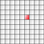
Even within grids, you have a choice of tiles, edges, and vertices[3] for movement. Tiles are the default choice, especially for games in which units only move to the center of a tile. In this diagram, the unit at A can move to any of the spots marked B. You may also wish to allow diagonal movement, with the same or higher movement cost.
If you’re using grids for pathfinding, your units are not constrained to grids, and movement costs are uniform, you may want to straighten the paths by moving in a straight line from one node to a node far ahead when there are no obstacles between the two.
Edge movement#
If your units can move anywhere within a grid space, or if the tiles are large, think about whether edges or vertices would be a better choice for your application.
A unit usually enters a tile at one of the edges (often in the middle) and exits the tile at another edge. With pathfinding on tiles, the unit moves to the center of the tile, but with pathfinding on edges, the unit will move directly from one edge to the other. I wrote a java applet demo of road drawing between edges[4]; that might help illustrate how edges can be used. [Most browser will not run applets as of 2021.]
Vertex movement#
Obstacles in a grid system typically have their corners at vertices. The shortest path around an obstacle will be to go around the corners. With pathfinding on vertices, the unit moves from corner to corner. This produces the least wasted movement, but paths need to be adjusted to account for the size of the unit.
Polygonal maps#
The most common alternative to grids is to use a polygonal representation. If the movement cost across large areas is uniform, and if your units can move in straight lines instead of following a grid, you may want to use a non-grid representation. You can use a non-grid graph for pathfinding even if your game uses a grid for other things.
Here’s a simple example of one kind of polygonal map representation. In this example, the unit needs to move around two obstacles:

Imagine how your unit will move in this map. The shortest path will be between corners of the obstacles. So we choose those corners (red circles) as the key “navigation points” points to tell A* about; these can be computed once per map change. If your obstacles are aligned on a grid, the navigation points will be aligned with the vertices of the grid. In addition, the start and end points for pathfinding need to be in the graph; these are added once per call to A*.
In addition to the navigation points, A* needs to know which points are connected. The simple algorithm is to build a visibility graph[5]: pairs of points that can be seen from each other. The simple algorithm may be fine for your needs, especially if the map doesn’t change during gameplay, but you may need a more sophisticated algorithm if the simple one is too slow. In addition, since we have added the start and end navigation points to the graph, we check line of sight from those to existing vertices and each other, and add edges where needed.
The third piece of information A* needs is travel times between the points. That will be manhattan distance or diagonal grid distance if your units move on a grid, or straight line distance if they can move directly between the navigation points.
A* will then consider paths from navigation point to navigation point. The pink line is one such path. This is much faster than looking for paths from grid point to grid point, when you have only a few navigation points, instead of lots of grid locations. When there are no obstacles in the way, A* will do very well—the start point and end point will be connected by an edge, and A* will find that path immediately, without expanding any other navigation points. Even when there are obstacles to consider, A* will jump from corner to corner until it finds the best path, which will still be much faster than looking for a path from a grid location to another.
Wikipedia has more about visibility graphs[6] from the robotics literature. This slide deck[7] is a nice introduction as well.
Managing complexity#
The above example was rather simple and the graph is reasonable. In some maps with lots of open areas or long corridors, a problem with visibility graphs becomes apparent. A major disadvantage of connecting every pair of obstacle corners is that if there are N corners (vertices), you have up to N2 edges. This example demonstrates the problem:

These extra edges primarily affect memory usage. Compared to grids, these edges provide “shortcuts” that greatly speed up pathfinding. There are algorithms for simplifying the graph by removing redundant edges. However, even after removing redundancies, there will still be a large number of edges.
Another disadvantage of the visibility graphs is that we have to add start/end nodes along with their new edges to the graph for every invocation of A*, and then remove them after we find a path. The nodes are easy to add but adding edges requires line of sight from the new nodes to all existing nodes, and that can be slow in large maps. One optimization is to only look at nearby nodes. Another option is to use a reduced visibility graph that removes the edges that aren’t tangent to both vertices (these will never be in the shortest path).
Navigation Meshes#
Instead of representing the obstacles with polygons, we can represent the walkable areas with non-overlapping polygons, also called a navigation mesh. The walkable areas can have additional information attached to them (such as “requires swimming” or “movement cost 2”). Obstacles don’t need to be stored in this representation.
The previous example becomes this:

We can then treat this much like we treat a grid. As with a grid, we have a choice of using polygon centers, edges, or vertices as navigation points.
Polygon movement#
As with grids, the center of each polygon provides a reasonable set of nodes for the pathfinding graph. In addition, we have to add the start and end nodes, along with an edge to the center of the polygon we’re in. In this example, the yellow path is the what we’d find using a pathfinder through the polygon centers, and the pink path is the ideal path.

The visibility graph representation would produce the pink path, which is ideal. Using a navigation mesh makes the map manageable but the path quality suffers. We can make the path look better by smoothing it.
Polygon edge movement#
Moving to the center of the polygon is usually unnecessary. Instead, we can move through the edges between adjacent polygons. In this example, I picked the center of each edge. The yellow path is what we’d find with a pathfinder through the edge centers, and it compares pretty well to the ideal pink path.

You can pick more points along the edge to produce a better path, at increased cost.
Polygon vertex movement#
The shortest way around an obstacle is to go around the corner. This is why we used corners for the visibility graph representation. We can use vertices with navigation meshes:

There’s only one obstacle in the way in this example. When we need to go around the obstacle, the yellow path goes through a vertex, as the pink (ideal) path does. However, whereas the visibility graph approach would have a straight line from the start point to the corner of the obstacle, the navigation mesh adds some more steps. These steps typically should not go through vertices, so the path looks unnatural, with “wall hugging” behavior.
Hybrid movement#
There aren’t any restrictions on what parts of each polygon can be made into navigation points for pathfinding. You can add multiple points along an edge, and the vertices are good points too. Polygon centers are rarely useful. Here’s a hybrid scheme that uses both the edge centers and vertices:

Note that to get around the obstacle, the path goes through a vertex, but elsewhere, it can go through edge centers.
Path smoothing#
Path smoothing is fairly easy with the resulting paths, as long as the movement costs are constant. The algorithm is simple: if there’s line of sight from the navigation point i to point i+2, remove point i+1. Repeat this until there is no line of sight between adjacent points in the path.
What will be left is only the navigation points that go around the corners of obstacles. These are vertices of the navigation mesh. If you use path smoothing, there’s no need to use edge or polygon centers as navigation points; use only the vertices.
In the above examples, path smoothing would turn the yellow path into the pink one. However, the pathfinder has no knowledge of these shorter paths, so its decisions won’t be optimal. Shortening the path found in an approximate map representation (navigation meshes) will not always produce paths that are as good as those found in a more exact representation (visibility graphs).
Hierarchical#
A flat map has but one level in its representation. It’s rare for games to have only one level—often there is a “tile” level and then a “sub-tile” level in which objects can move within a tile. However, it’s common for pathfinding to occur on only the larger level. You can also add higher levels such as “rooms”.
Having fewer nodes in the map representation is better for pathfinding speed. One way to reduce the problem is to have multiple levels of searching. For example, to get from your home to a location in another city, you would find a path from your chair to your car, from the car to the street, from the street to a freeway, from the freeway to the edge of the city, from there to the other city, then to a street, to a parking lot, and finally to the door of the destination building. There are several levels of searching here:
- At the street level, you are concerned with walking from one location to a nearby location, but you do not go out on the street.
- At the city level, you go from one street to another until you find the freeway. You do not worry about going into buildings or parking lots, nor do you worry about going on freeways.
- At the state level, you go from one city to another on the freeway. You do not worry about streets within cities until you get to your destination city.
Dividing the problem into levels allows you to ignore most of your choices. When moving from city to city, it is quite tedious to consider every street in every city along the way. Instead, you ignore them all, and only consider freeways. The problem becomes small and manageable, and solving it becomes fast.
A hierarchical map has many levels in its representation. A heterogenous hierarchy typically has a fixed number of levels, each with different characteristics. Ultima V, for example, has a “world” map, on which are cities and dungeons. You can enter a city or dungeon and be in a second map level. In addition, there are “layers” of worlds on top of one another, making for a three-level hierarchy. The levels can be of different types (tile grids, visibility, navigation mesh, waypoints). A homogeneous hierarchy has an arbitrary number of levels, each with the same characteristics. Quad trees and oct trees can be considered to be homogeneous hierarchies.
In a hierarchical map, pathfinding may occur on several levels. For example, if a 1024x1024 world was divided into 64x64 “zones”, it may be reasonable to find a path from the player’s location to the edge of the zone, then from zone to zone until reaching the desired zone, then from the edge of that zone to the desired location. At the coarser levels, long paths can be found more easily because the pathfinder does not consider all of the details. When the player actually walks across each zone, the pathfinder can be invoked again to find a short path through that zone. By keeping the problem size small, the pathfinder can run quicker.
You can use multiple levels with graph-searching algorithms such as A*, but you do not need to use the same algorithm at each level. For small levels, you may be able to precompute the shortest path between all pairs of nodes (using Floyd-Warshall or other algorithms). In general, pathfinding in a hierarchical map will not produce optimal paths, but they are usually close.
A similar approach is to use varying resolution. First, plot a path with low resolution. As you get closer to a point, refine the path with a higher resolution. This approach can be used with path splicing to avoid moving obstacles.
Some papers to read: Near-Optimal Hierarchical Pathfinding (HPA*)[8] builds a two-level hierarchy on a grid (or read the paper[9]), Pathfinding for Dragon Age:Origins[10] (2012) explains several hierarchical approaches used in a commercial game, Ultrafast shortest-path queries with linear-time preprocessing[11] by using “transit nodes” for a road graph [PDF], TRANSIT Routing on Video Game Maps[12] (2012) [PDF], Hierarchical A*: Searching Abstraction Hierarchies Efficiently[13], Route Planning in Road Networks[14] (Dominic Schultes’s PhD thesis), Hierarchical Annotated A* (part 1[15] and part 2[16] and source code[17]).
Wraparound maps#
If your world is spherical or toroidal, then objects can “wrap” around
from one end of the map to the other. The shortest path could lie in
any direction, so all directions must be explored. If using a grid,
you can adapt the heuristic to consider
wrapping around. Instead of abs(x1 - x2) you can use min(abs(x1 - x2), (x1+mapsize) - x2, (x2+mapsize) - x1). This will
take the min of three options: either staying on the map
without wrapping, wrapping when x1 is on the left side, or
wrapping when x2 is on the left side. You’d do the same for
each axis that wraps. Essentially you calculate the heuristic assuming
that the map is adjacent to copies of itself.
Connected Components#
In some game maps, there’s no path between the source and destination. If you ask A* to find a path, it will end up exploring a large subset of the graph before it determines that there’s no path. If the map can be analyzed beforehand, mark each of the connected subgraphs[18] with a different marker. Then, before looking for a path, check if the source and destination are both in the same subgraph. If not, then you know there’s no path between them. Hierarchical pathfinding can also be useful here, especially if there are one way edges between subgraphs.
Road maps#
If your units can only move on roads, you may want to consider giving A* the road and intersection information. Each intersection will be a node in the graph, and each road will be an edge. A* will find paths from intersection to intersection, which is much faster than using a grid representation.
For some applications, your units may not start and end on intersections. To handle this case, each time you run A*, you will need to modify the node/edge graph (this is the same technique we use with visibility graph and navigation mesh map representations). Add the starting and ending points as new nodes, and add edges between these points and their nearest intersections. After pathfinding, remove these extra nodes and edges from the graph so that the graph is ready to be used for the next invocation of A*.

In this diagram, the intersections become nodes in the pathfinding graph for A*. The edges are the roads between the nodes, and these edges should be given the driving distance along each road. In the “roads as edges” framework, you can incorporate one-way roads as unidirectional edges in the graph.
If you want to assign costs to turning, you can extend the framework a bit: instead of nodes being locations, consider nodes to be a <location, direction> pair (a point in state space), where the direction indicates what direction you were facing when you arrived at that location. Replace edges from P to Q with edges from <P, dir> to <Q, dir> to represent a straight drive, and from <P, dir1> to <P, dir2> to represent a “turn”. Each edge represents either a straight drive or a turn, but not both. You can then assign costs to the edges representing turns.
The neighbors function would look something like this:
function neighbors(p):
     let res = new List()
     if p.dir == 'east':
        res.append({x: p.x+1, y: p.y, dir: 'east'}  // straight
        res.append({x: p.x,   y: p.y, dir: 'south'} // turn right
        res.append({x: p.x,   y: p.y, dir: 'north'} // turn left
     if p.dir == 'north':
        …
     if p.dir == 'west'':
        …
     if p.dir == 'south':
        …
     return res
If you also need to take into account turn limitations, such as “only right turns”, you can use a variation of this framework in which the two types of edges are always combined. Each edge represents an optional turn followed by a straight drive. In this framework, you can represent restrictions like “you can only turn right”: include an edge from <P, north> to <Q, north> for driving straight, and an edge from <P, north> to <R, east> for the right turn followed by a drive, but don’t include <P, north> to anything west, because that would mean a left turn, and don’t include anything south, because that would mean a U-turn.
In this framework, you can model a large city downtown, in which you have one-way streets, turn restrictions at certain intersections (often prohibiting U-turns and sometimes prohibiting left turns), and turn costs (to model slowing down and waiting for pedestrians before you turn right). Compared to grid maps, A* can find paths in road graphs environment fairly quickly, because there are few choices to make at each graph node, and there are relatively few nodes in the map.
For large scale road maps, be sure to read Goldberg and Harrelson’s paper[19] on ALT (A*, Landmarks, Triangle inequality) (PDF is here[20], or this paper[21].) It was also published SODA 2005[22].
Related topic: Dubins paths[23].
Skip links#
A pathfinding graph constructed from a grid typically assigns a vertex to each location and an edge to each possible movement from a location to an adjacent location. The edges are not constrained to be between adjacent vertices. A “skip link” or “shortcut link” is an edge between non-adjacent vertices. It serves to shortcut the pathfinding process.
What should the movement cost be for a skip link? There are two approaches:
- Make the cost match the movement cost of the best path. This preserves nice properties of A*, like finding optimal paths. To give A* a nudge in the right direction, break the tie between the skip link and the regular links by reducing the skip link’s cost by 1% or so.
- Make the cost match the heuristic cost. This makes a much stronger impact on performance but you give up optimal paths.
Adding skip links is an approximation of a hierarchical map. It takes less effort but can often give you many of the same performance benefits.
For dungeon room-and-corridor grid maps, Rectangular Symmetry Reduction and Jump Point Search[24] offer two different ways to build skip links. Rectangular Symmetry Reduction statically builds additional edges (which they call macro edges) and then uses standard graph search; Jump Point Search dynamically builds longer edges as part of the graph search algorithm. For road maps and other types of graphs Contraction Hierarchies[25] are worth looking at; see this paper[26] or this library[27]. When I wrote this page in 1997 I didn’t know about contraction hierarchies, or I would’ve used that terminology instead of making up the term “skip links”.
Waypoints#
A waypoint is a point along a path. Waypoints can specific to each path or be part of the game map. Waypoints can be entered manually or computed automatically. In many real-time strategy games, players can manually add path-specific waypoints by shift-clicking. When automatically computed along a path, waypoints can be used to compress the path representation. Map designers can manually add waypoints (or “beacons”) to a map to mark locations that are along good paths or an algorithm can be used to automatically mark waypoints on a map.
Since the goal of skip links is to make pathfinding faster when those links are used, skip links should be placed between designer-placed waypoints. This will maximize their benefit.
If there are not too many waypoints, the shortest paths between each pair of waypoints can be precomputed beforehand (using an all-pairs shortest path algorithm, not A*). The common case will then be a unit following its own path until it reaches a waypoint, and then it will follow the precomputed shortest path between waypoints, and finally it will get off the waypoint highway and follow its own path to the goal.
Using waypoints or skip links with false costs can lead to suboptimal paths. It is sometimes possible to smooth out a bad path in a post-processing step or in the movement algorithm.
Graph Format Recommendations#
Start by pathfinding on the game world representation you already use. If that’s not satisfactory, consider transforming the game world into a different representation for pathfinding.
In many grid games, there are large areas of maps that have uniform movement costs. A* doesn’t “know” this, and wastes effort exploring them. Creating a simpler graph (navigation mesh, visibility graph, or hierarchical representation of the grid map) can help A*.
The visibility graph representation produces the best paths when movement costs are constant, and allows A* to run rather quickly, but can use lots of memory for edges. Grids allow for fine variation in movement costs (terrain, slope, penalties for dangerous areas, etc.), use very little memory for edges, but use lots of memory for nodes, and pathfinding can be slow. Navigation meshes are in between. They work well when movement costs are constant in a larger area, allow for some variation in movement costs, and produce reasonable paths. The paths are not always as short as with visibility graph representation, but they are usually reasonable. Hierarchical maps use multiple levels of representation to handle both coarse paths over long distances and detailed paths over short distances.
You can read more about navigation meshes in this well-illustrated article[28]. Note that the article is comparing (a) keeping walkable polygons to keeping only navigation points, and (b) moving along vertices to moving along polygon centers. These are mostly orthogonal. Keeping the walkable polygons is nice for dynamically adjusting the path later, but not needed in all games. Using vertices is better for obstacle avoidance, and if you’re using path smoothing it won’t negatively affect path quality. Without path smoothing, edges might perform better, so consider either edges or edges+vertices.
An alternative to building a separate non-grid representation of a grid map is to use a variant of A* that better understands grid maps with uniform costs. See Jump Point Search to speed up A* on square grids and any angle movement to generate non-grid movement on a grid.